
Most tutorials hand you
sklearn.cluster.KMeansand call it a day. This one builds it from nothing, watches it think, and shows you exactly what the algorithm is doing at every step — because understanding it is worth more than importing it.
What K-Means Actually Is
Before a single line of code, let’s get the idea straight.
You have a pile of data points. No labels. No categories. Just points scattered in space. K-Means looks at that pile and asks: if I had to draw K circles around this data, where would I put them so that every point is as close as possible to the centre of its circle?
That’s it. That’s the whole algorithm. Find K centres — called centroids — such that every point belongs to its nearest centroid, and the total distance from every point to its centroid is minimised.
The elegant part is how it solves this. It doesn’t solve it perfectly. It solves it iteratively — guessing, adjusting, guessing again — until it stops changing. And when it stops, it’s found a solution good enough to be useful.
Here’s the loop it runs:
- Place K centroids somewhere in the space, initially at random.
- Assign every data point to the nearest centroid. These become the clusters.
- Move each centroid to the mean position of all the points assigned to it.
- If any centroid moved, go back to step 2. If nothing moved, you’re done.
That’s the complete algorithm. Two operations repeated until convergence: assign and update.
The Dataset
We’re going to use the Iris dataset. It’s built into scikit-learn, it’s clean, and it has natural clusters that K-Means can find — which means we can actually verify whether our implementation is working.
The Iris dataset has 150 samples, four features (sepal length, sepal width, petal length, petal width) and three species. We’ll use only two features at a time so we can visualise everything in 2D.
We’ll also generate a synthetic blob dataset using sklearn.datasets.make_blobs for the first experiments, because blobs are perfectly shaped clusters and make it easy to verify the algorithm is behaving correctly before testing it on real data.
Install what you need if you don’t have it:
pip install numpy matplotlib scikit-learn pillow
Setting Up
import numpy as np
import matplotlib.pyplot as plt
import matplotlib.animation as animation
from sklearn.datasets import make_blobs, load_iris
from sklearn.preprocessing import StandardScaler

# Reproducibility
np.random.seed(42)
The np.random.seed(42) call matters. K-Means starts by placing centroids randomly. Without a fixed seed, every run produces different initial positions, which sometimes leads to different final clusters. Fixing the seed makes the results reproducible while you’re learning.
Generating the Synthetic Data
Start with blobs. They’re forgiving and make the algorithm easy to debug.
# Generate 300 points in 3 natural clusters
X, y_true = make_blobs(
    n_samples=300,
    centers=3,
    cluster_std=0.8,
    random_state=42
)

plt.figure(figsize=(8, 6))
plt.scatter(X[:, 0], X[:, 1], c='#cccccc', s=40, alpha=0.7, edgecolors='white', linewidths=0.5)
plt.title('Raw Data — No Labels', fontsize=14)
plt.xlabel('Feature 1')
plt.ylabel('Feature 2')
plt.tight_layout()
plt.show()
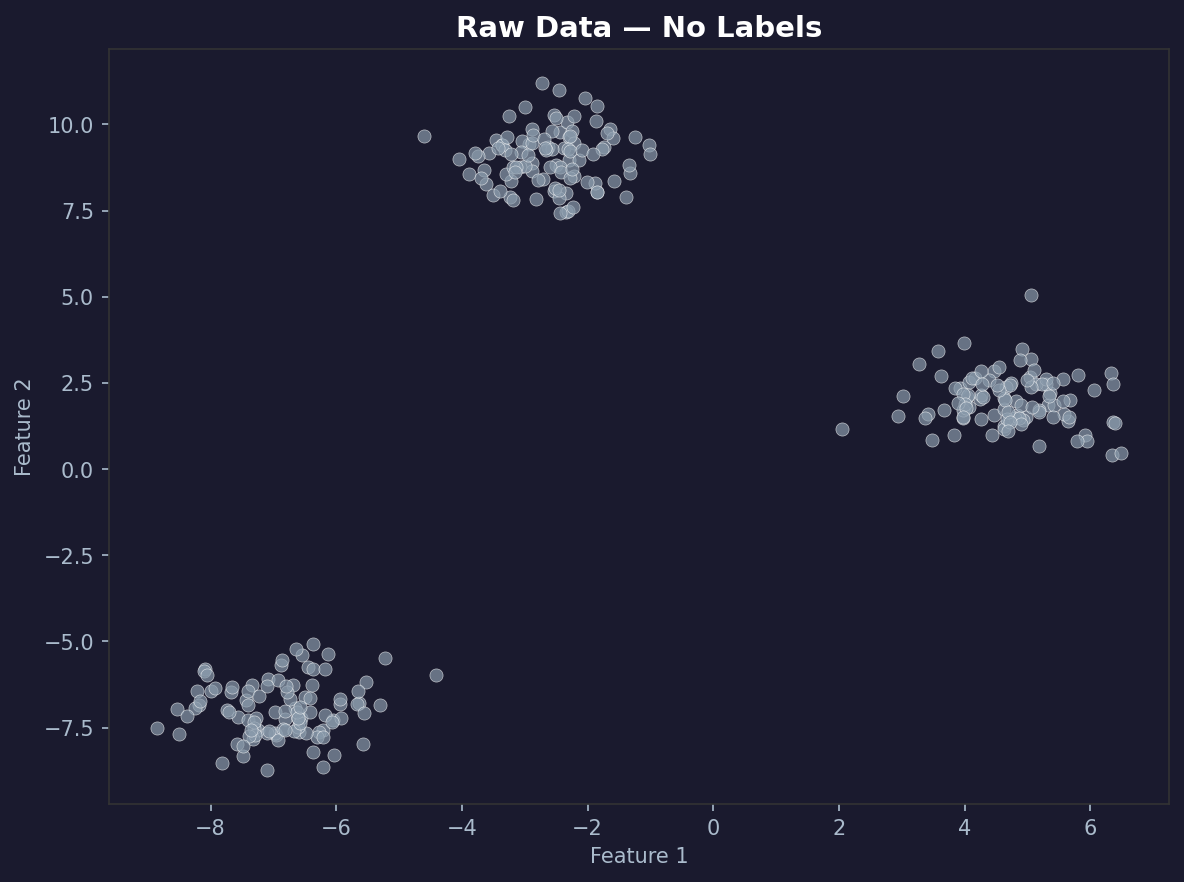
You should see three distinct blobs. The algorithm doesn’t know they’re three blobs. It’s going to figure that out on its own.
Building K-Means From Scratch
Now the actual implementation. We’ll build it as a class with methods that match the conceptual steps exactly.
class KMeans:
    def __init__(self, k=3, max_iterations=100, tolerance=1e-4):
        self.k = k
        self.max_iterations = max_iterations
        self.tolerance = tolerance
        self.centroids = None
        self.labels = None
        self.history = []  # stores (centroids, labels) at every iteration

    def initialise_centroids(self, X):
        # Pick K random data points as starting centroids.
        # Using actual data points avoids placing centroids in empty regions.
        indices = np.random.choice(len(X), self.k, replace=False)
        return X[indices].copy()

    def assign_clusters(self, X, centroids):
        # For every point in X, find the nearest centroid.
        # X shape: (n_samples, n_features)
        # centroids shape: (k, n_features)
        # distances shape: (n_samples, k)
        distances = np.sqrt(
            ((X[:, np.newaxis, :] - centroids[np.newaxis, :, :]) ** 2).sum(axis=2)
        )
        return np.argmin(distances, axis=1)

    def update_centroids(self, X, labels):
        # Move each centroid to the mean of its assigned points.
        # If a cluster is empty, reinitialise to a random data point.
        new_centroids = np.zeros((self.k, X.shape[1]))
        for k in range(self.k):
            points_in_cluster = X[labels == k]
            if len(points_in_cluster) == 0:
                new_centroids[k] = X[np.random.choice(len(X))]
            else:
                new_centroids[k] = points_in_cluster.mean(axis=0)
        return new_centroids

    def has_converged(self, old_centroids, new_centroids):
        movement = np.sqrt(((new_centroids - old_centroids) ** 2).sum(axis=1))
        return movement.max() < self.tolerance

    def fit(self, X):
        self.centroids = self.initialise_centroids(X)

        for iteration in range(self.max_iterations):
            self.labels = self.assign_clusters(X, self.centroids)
            self.history.append({
                'iteration': iteration,
                'centroids': self.centroids.copy(),
                'labels': self.labels.copy()
            })
            new_centroids = self.update_centroids(X, self.labels)

            if self.has_converged(self.centroids, new_centroids):
                self.centroids = new_centroids
                self.labels = self.assign_clusters(X, self.centroids)
                self.history.append({
                    'iteration': iteration + 1,
                    'centroids': self.centroids.copy(),
                    'labels': self.labels.copy()
                })
                print(f"Converged after {iteration + 1} iterations.")
                break

            self.centroids = new_centroids

        return self

    def predict(self, X):
        return self.assign_clusters(X, self.centroids)

    def inertia(self, X):
        # Total within-cluster sum of squared distances. Lower is better.
        total = 0
        for k in range(self.k):
            points = X[self.labels == k]
            if len(points) > 0:
                total += ((points - self.centroids[k]) ** 2).sum()
        return total
Every method maps to one conceptual step. initialise_centroids is step one. assign_clusters is step two. update_centroids is step three. has_converged is step four. fit runs the loop.
The history list is what makes the visualisation possible. Every iteration, we snapshot exactly where the centroids are and which cluster every point belongs to.
Running the Algorithm
kmeans = KMeans(k=3, max_iterations=100)
kmeans.fit(X)

print(f"Number of iterations stored: {len(kmeans.history)}")
print(f"Final centroids:\n{kmeans.centroids}")
print(f"Final inertia: {kmeans.inertia(X):.2f}")
You should see something like:
Converged after 6 iterations.
Number of iterations stored: 7
Final inertia: 212.47
K-Means on clean blob data converges fast. Six iterations. On messier real-world data it takes longer, but the mechanism is identical.
Visualising Every Iteration
This is where it gets interesting. We stored the full history — now we can watch the algorithm think.
def plot_iteration(ax, X, centroids, labels, iteration, k):
    colors = ['#e74c3c', '#3498db', '#2ecc71', '#f39c12', '#9b59b6']
    ax.clear()
    for cluster in range(k):
        mask = labels == cluster
        ax.scatter(X[mask, 0], X[mask, 1], c=colors[cluster], s=35, alpha=0.6,
                   edgecolors='white', linewidths=0.3, label=f'Cluster {cluster + 1}')
    ax.scatter(centroids[:, 0], centroids[:, 1],
               c=[colors[i] for i in range(k)], s=250, marker='*',
               edgecolors='black', linewidths=1.5, zorder=5)
    ax.set_title(f'Iteration {iteration}', fontsize=13, fontweight='bold')
    ax.set_xlabel('Feature 1')
    ax.set_ylabel('Feature 2')
    ax.legend(loc='upper right', fontsize=9)

n_iters = len(kmeans.history)
cols = 3
rows = (n_iters + cols - 1) // cols

fig, axes = plt.subplots(rows, cols, figsize=(15, 5 * rows))
axes = axes.flatten()

for i, state in enumerate(kmeans.history):
    plot_iteration(axes[i], X, state['centroids'], state['labels'],
                   state['iteration'], kmeans.k)

for j in range(n_iters, len(axes)):
    axes[j].set_visible(False)

plt.suptitle('K-Means: Every Iteration', fontsize=16, fontweight='bold', y=1.02)
plt.tight_layout()
plt.savefig('kmeans_iterations.png', dpi=150, bbox_inches='tight')
plt.show()
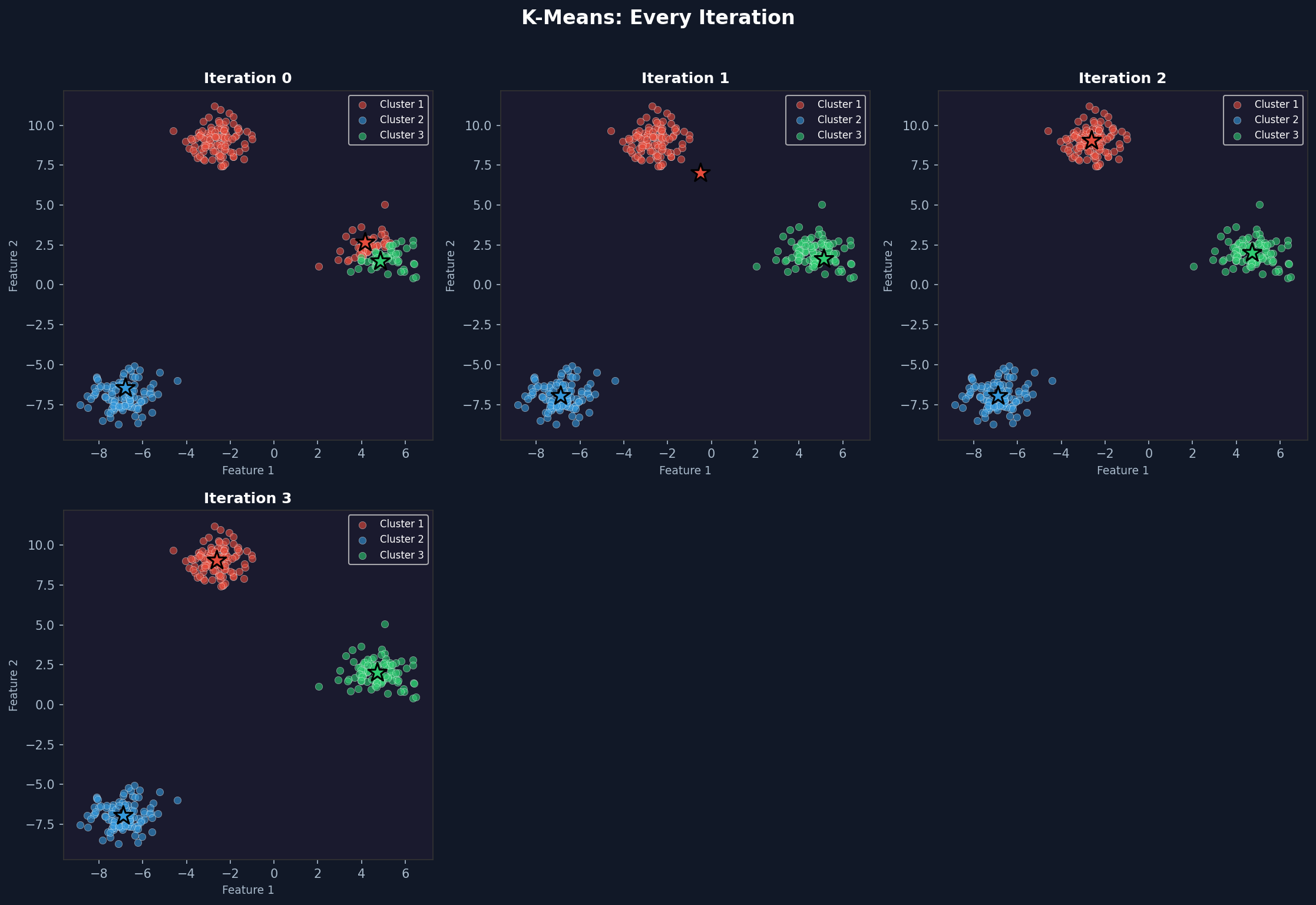
Iteration 0 shows the randomly placed centroids with an initial assignment that may look wrong. By iteration 2 or 3 the clusters start looking correct. By convergence they match the underlying blobs almost perfectly.
The star markers are the centroids. Watch them move toward the centre of each cluster across iterations. That movement is the algorithm learning.
Building an Animated Version
A static grid is informative. An animation makes it visceral. You can see the centroids drift, watch the boundaries shift, and feel the moment it locks in.
def create_animation(X, history, k, filename='kmeans_animation.gif'):
    colors = ['#e74c3c', '#3498db', '#2ecc71', '#f39c12', '#9b59b6']
    fig, ax = plt.subplots(figsize=(8, 6))

    def animate(frame):
        state = history[frame]
        centroids = state['centroids']
        labels = state['labels']
        ax.clear()
        ax.set_facecolor('#1a1a2e')
        fig.patch.set_facecolor('#1a1a2e')
        for cluster in range(k):
            mask = labels == cluster
            ax.scatter(X[mask, 0], X[mask, 1], c=colors[cluster], s=40, alpha=0.7,
                       edgecolors='white', linewidths=0.3)
        ax.scatter(centroids[:, 0], centroids[:, 1],
                   c='white', s=300, marker='*', edgecolors='black', linewidths=1.5, zorder=5)
        if frame > 0:
            prev_centroids = history[frame - 1]['centroids']
            for c in range(k):
                ax.annotate('', xy=centroids[c], xytext=prev_centroids[c],
                            arrowprops=dict(arrowstyle='->', color='white', lw=1.5, alpha=0.6))
        ax.set_title(f'Iteration {state["iteration"]}  |  K={k}',
                     fontsize=13, color='white', fontweight='bold')
        ax.tick_params(colors='white')
        for spine in ax.spines.values():
            spine.set_edgecolor('#444')

    anim = animation.FuncAnimation(fig, animate, frames=len(history), interval=800, repeat=True)
    anim.save(filename, writer='pillow', fps=1.2, dpi=100)
    plt.close()

create_animation(X, kmeans.history, k=3)
The white arrows show each centroid’s movement from the previous iteration. On the first frame, the arrows don’t appear. On every subsequent frame they trace the path each centroid took to get there. By the final frame, the arrows are tiny or invisible because convergence means the centroids barely moved.
Testing on the Iris Dataset
Synthetic blobs are easy. Real data is messier. The Iris dataset has three species with some overlap in the feature space — a proper test of what the algorithm actually does on data that doesn’t behave perfectly.
iris = load_iris()
X_iris = iris.data

# Use only petal length and petal width — these separate species most clearly
X_iris_2d = X_iris[:, 2:4]

# Standardise — K-Means uses Euclidean distance, so scale matters
scaler = StandardScaler()
X_iris_scaled = scaler.fit_transform(X_iris_2d)

kmeans_iris = KMeans(k=3, max_iterations=100)
kmeans_iris.fit(X_iris_scaled)

print(f"Iris convergence: {len(kmeans_iris.history)} iterations")
print(f"Iris inertia: {kmeans_iris.inertia(X_iris_scaled):.4f}")
The scaling step is important. K-Means calculates Euclidean distance, which means features with larger numerical ranges dominate the distance calculation. Standardising puts every feature on the same scale so the algorithm treats them equally.
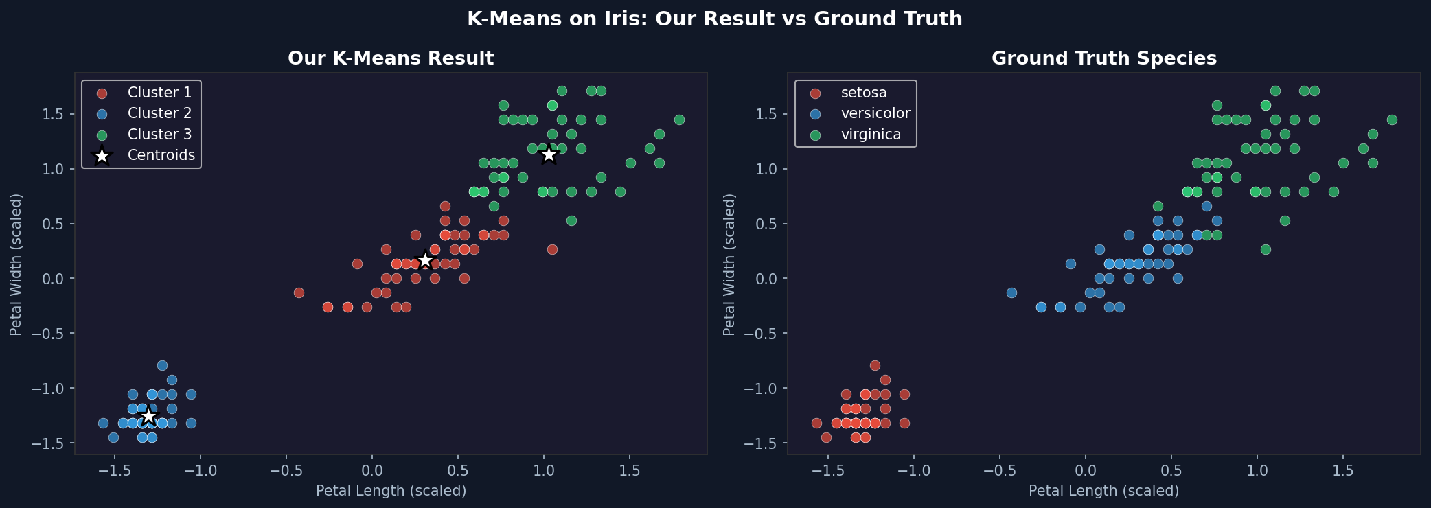
The result won’t be perfect. Setosa separates cleanly. Versicolor and Virginica overlap slightly in the petal feature space, so K-Means will misclassify some of those boundary points. That’s expected and honest — K-Means assumes spherical clusters of similar size. When the real clusters aren’t perfectly spherical, it approximates.
Finding the Right K — The Elbow Method
One of the most common questions with K-Means: how do you choose K?
The elbow method plots inertia against K. As K increases, inertia always decreases — more clusters means every point is closer to its nearest centroid. But after a certain point, adding more clusters gives diminishing returns. That point of diminishing returns looks like an elbow in the plot.
def elbow_plot(X, k_range=range(1, 11), n_runs=3):
    inertias = []
    for k in k_range:
        best_inertia = float('inf')
        for _ in range(n_runs):
            km = KMeans(k=k, max_iterations=100)
            km.fit(X)
            current_inertia = km.inertia(X)
            if current_inertia < best_inertia:
                best_inertia = current_inertia
        inertias.append(best_inertia)
        print(f"K={k}: inertia={best_inertia:.2f}")

    fig, ax = plt.subplots(figsize=(9, 5))
    ax.plot(list(k_range), inertias, 'o-', color='#3498db', linewidth=2.5, markersize=8)
    ax.fill_between(list(k_range), inertias, alpha=0.1, color='#3498db')
    ax.set_xlabel('Number of Clusters (K)', fontsize=12)
    ax.set_ylabel('Inertia', fontsize=12)
    ax.set_title('Elbow Method — Finding the Optimal K', fontsize=14, fontweight='bold')
    ax.set_xticks(list(k_range))
    ax.grid(True, alpha=0.3)
    plt.tight_layout()
    plt.savefig('elbow_plot.png', dpi=150, bbox_inches='tight')
    plt.show()
    return inertias

inertias = elbow_plot(X)
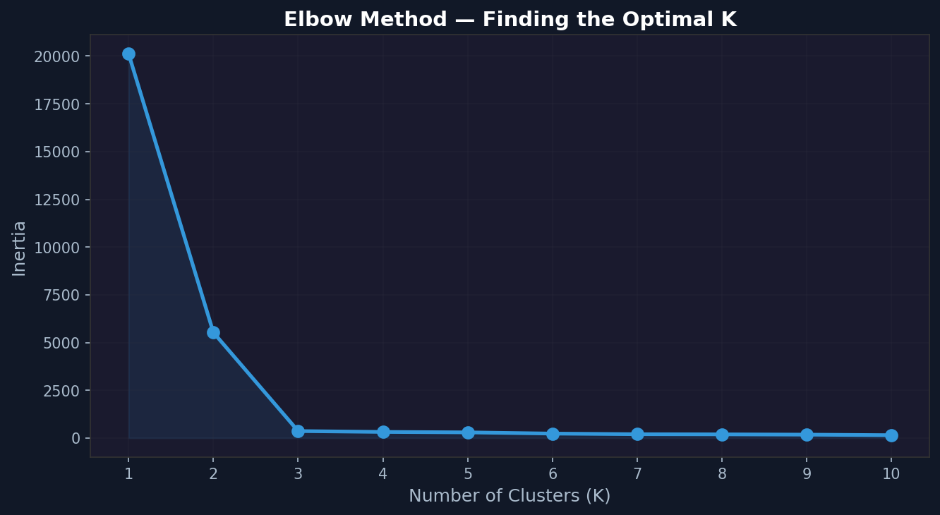
For the blob dataset, the elbow should appear clearly at K=3. For the Iris data, run the same function with X_iris_scaled. The elbow appears around K=3 — a satisfying confirmation that the method works.
Why Random Initialisation Is a Problem
K-Means isn’t guaranteed to find the global optimum. It finds a local optimum, and which local optimum it finds depends on where the centroids started.
This is worth demonstrating directly:
print("Running K-Means 5 times with different random seeds:\n")
results = []
for seed in range(5):
    np.random.seed(seed)
    km = KMeans(k=3, max_iterations=100)
    km.fit(X)
    inertia = km.inertia(X)
    results.append(inertia)
    print(f"Seed {seed}: inertia = {inertia:.2f}, iterations = {len(km.history)}")

print(f"\nBest:  {min(results):.2f}")
print(f"Worst: {max(results):.2f}")
print(f"Difference: {max(results) - min(results):.2f}")
On clean blob data the difference will be small. On messier data like Iris, you’ll see more variation. The solution in production is to run K-Means multiple times and keep the result with the lowest inertia — which is exactly what scikit-learn does with its n_init parameter.
Comparing With scikit-learn
Now verify our implementation produces results consistent with the library version:
from sklearn.cluster import KMeans as SklearnKMeans

sklearn_km = SklearnKMeans(n_clusters=3, n_init=10, random_state=42)
sklearn_km.fit(X)

np.random.seed(42)
our_km = KMeans(k=3)
our_km.fit(X)

print(f"sklearn inertia:  {sklearn_km.inertia_:.2f}")
print(f"our inertia:      {our_km.inertia(X):.2f}")

print(f"\nsklearn centroids:\n{sklearn_km.cluster_centers_}")
print(f"\nour centroids:\n{our_km.centroids}")
The inertia values won’t be identical — sklearn uses K-Means++ initialisation by default, which is smarter than pure random and consistently finds better starting positions. But they should be in the same range. Our centroids will be close to sklearn’s, possibly with cluster indices swapped (cluster 0 in ours might be cluster 2 in sklearn — the labelling is arbitrary).
What K-Means Gets Wrong
The algorithm has real limitations. Understanding them is as important as understanding the algorithm itself.
Assumes spherical clusters. K-Means minimises Euclidean distance, which implicitly assumes clusters are roughly circular. Elongated clusters, crescent shapes, or clusters of different densities confuse it badly.
Sensitive to scale. Features with large numerical ranges dominate the distance calculation. Always standardise before running K-Means.
K must be specified in advance. You have to tell it how many clusters to find. The elbow method helps but doesn’t always produce a clean answer on real-world data.
Sensitive to initialisation. As demonstrated above, different starting points can produce different final clusters. Running multiple times and keeping the best result is standard practice.
Outliers distort centroids. Because centroids are means, a single extreme outlier can pull a centroid far from the actual cluster. Remove or investigate outliers before clustering.
The Full Picture
What we built does the same thing as scikit-learn’s KMeans — it just does it without the optimisations. The core loop is identical: initialise, assign, update, repeat until convergence.
The visualisation history is something the library doesn’t give you. Watching the centroids move and the cluster boundaries shift makes the algorithm intuitive in a way that no diagram or explanation quite manages. Run it on a few different datasets and the behaviour becomes predictable — you start to know, before it finishes, roughly where the centroids will end up.
That intuition is what makes you effective when the library version produces unexpected results. You know what it’s doing. You know why it might be struggling. And you know which of its limitations applies to your specific data.
That’s the value of building it yourself.
Mohun Shakeel Ahmad — Software Engineer at Spoon Consulting / SharinPix. MSc Data Science (Distinction), Sunway University. BSc Computer Science (First Class Honours), University of Mauritius. Writing about software engineering, data science and AI for practitioners.